Individual-Level Parameters
| Related Online Training modules | |
|---|---|
| Individual-Level Parameters | |
| Generally it is best to access online training from within Q by selecting Help > Online Training |
Most analyses in Q are, to some extent, averages of one form or another.[note 1] However, from time-to-time it is useful to examine the raw data or to use it to create a simulator. When reviewing an Experiment, examination of the raw data is not so useful, as we are generally interested how the coefficients differ by respondents, rather than the raw data itself.
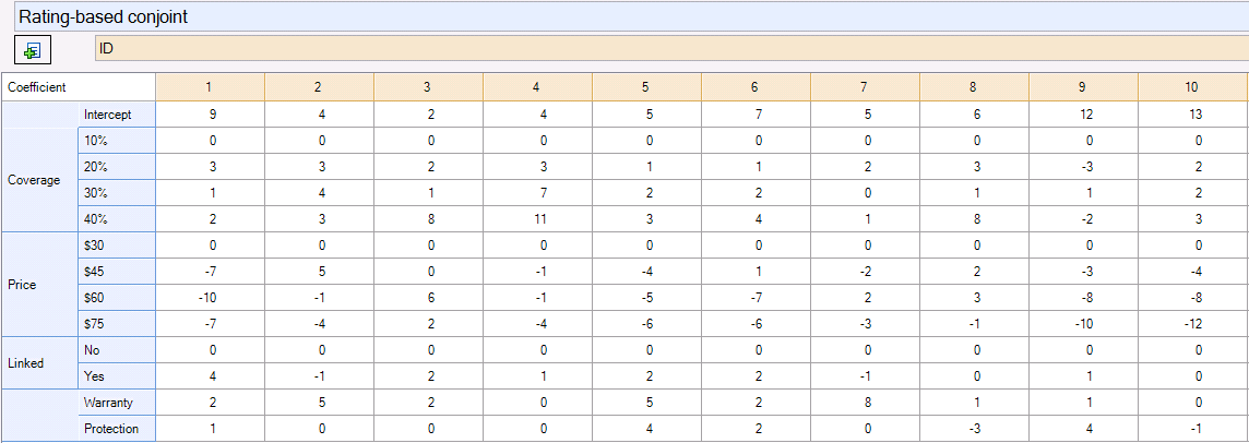
One way of understanding how coefficients differ by respondents is to estimate a separate model for every respondent. This can be done by crosstabbing an Experiment question by a Pick One variable which contains a unique identifier. The table below, for example, shows coefficients estimated for the first 10 respondents from the Discount.Q project.
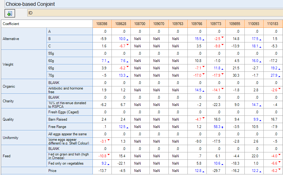
The table above, for example, shows coefficients estimated for the first 10 respondents from the Conjoint Analysis Case Study. The table below shows the results for the first 10 respondents from the Discrete Choice Experiment Case Study. It reveals a number of problems. First, the eighth respondent has no coefficients; this is because the way that this experiment was designed, it was impossible to obtain parameters for individual respondents.[note 2] Second, many of the parameter estimates are counter-intuitive; for example, the third respondent prefers 55g to 60g eggs; an examination of the standard errors (Statistics - Cells) shows that this is because many of the parameters are not identified. When the coefficients estimated from the conjoint analysis (shown above) are more closely examined, they also reveal inexplicable patterns – we can see, for example, that “irrational” price coefficients have been estimated for most respondents (we would expect to see that people would have lower coefficients for higher prices).
The nonsensical results obtained by estimating models for individual respondents should not be interpreted as meaning that the data is poor; rather, it likely means that the idea of estimating a model for a single respondent is too optimistic. The solution to this problem is to use shrinkage estimators, which assign each respondent a coefficient by using data from other similar respondents (i.e., similar in terms of how they reacted to the experiment).
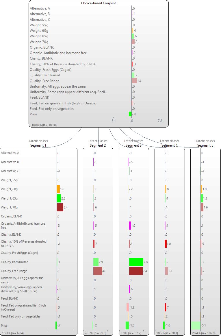
Q has a variety of alternative shrinkage estimates. The first step is to create segmentation tree of the Experiment, either splitting by individuals (Latent Class Analysis), splitting by questions (Trees) or a combination of the two. When this is done, within the dialog box containing text outputs, Q presents a table showing the shrinkage obtained if computing coefficients for each respondent using the model. Looking at Price, for example, this table shows us that this the latent class model estimates that the true standard deviation in the population is 2.010, but if we attempt to compute coefficients for each respondent, the standard deviation that we can compute using this data is slightly smaller (1.910), which is the “shrinkage”. The last column shows the ratio between the sample variance and the population variance, which is an estimate of the degree of shrinkage. The tree that is created is shown below.
Individual-level parameter shrinkage
                                                Population St Dev  Sample St Dev  Variance explained(%)
B                                                            .204           .181                 78.726
C                                                            .246           .237                 92.194
60g                                                          .531           .495                 86.849
65g                                                          .778           .710                 83.296
70g                                                         1.173          1.039                 78.382
Antibiotic and hormone free                                  .255           .241                 89.433
10% of Revenue donated to RSPCA                              .343           .294                 73.492
Barn Raised                                                 2.186          2.027                 85.909
Free Range                                                  2.389          2.257                 89.276
Some eggs appear different (e.g. Shell Colour)               .227           .207                 82.815
Fed on grain and fish (high in Omega)                        .491           .434                 78.054
Fed only on vegetables                                       .180           .156                 75.028
Price                                                       2.010          1.910                 90.266
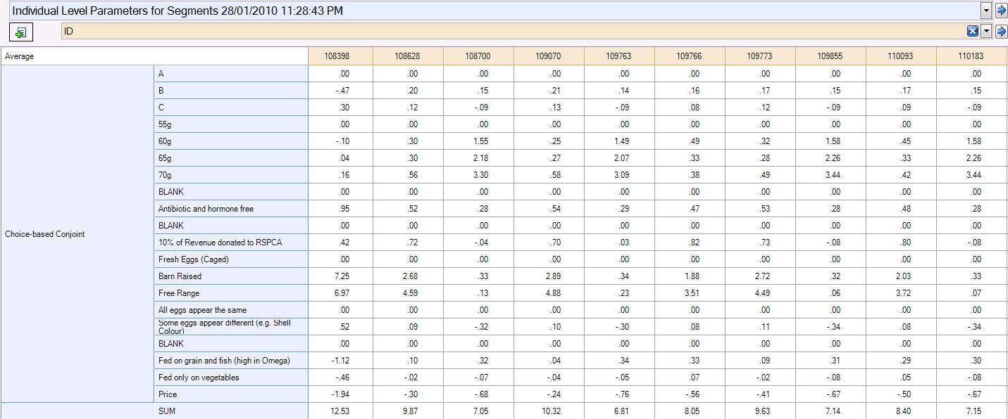
The second step is to right-click on the tree and select Save Individual-Level Parameter Means and Standard Deviations, which creates a Number - Multi question that contains coefficients for all the respondents. The estimated parameters are shown below (obtained by crosstabbing with ID); although there are still some inconsistencies, by and large the estimated coefficients are much more plausible.
Q also has some more complex models that can be used for estimating individual-level parameters from Experiments. We can get Q to estimate a normal distribution within each latent class by changing the option Distribution assumption from Finite.
When Multivariate Normal – Spherical is selected, the model assumes all coefficients have identical standard deviations and are uncorrelated (i.e., that an individual’s coefficient on one attribute level is unrelated to any other). When Multivariate Normal – Diagonal is selected, the model estimates separate standard deviations for each coefficient and assumes that the coefficients are uncorrelated. Multivariate Normal – Block Diagonal estimates correlations between different levels of the same attribute. Multivariate Normal – Full Covariance estimates correlations between all levels of all attributes. When the option Pool variance is checked, Q constrains the covariance matrix to be equal across all classes. The Multivariate Normal – Diagonal and Multivariate Normal – Full Covariance models where Pool variance is not checked are sometimes referred to as HB or Hierarchical Bayes.[note 3]
Scaling
Differences between segments or individuals can be difficult to interpret where the data has different levels of noise.[note 4] One solution to this problem is to rescale the utilities so that the range of utilities for each attribute has a maximum value of 100. This is best done in Excel.
Notes
Further reading: Latent Class Analysis Software


